Models and Methods III: Fit PSD Model by VI Algorithm

Introduction

We use the variational inference algorithm (VI) to fit the PSD model (Raj, Stephens, and Pritchard 2014).

PSD Model

Suppose we have \(I\) diploid individuals genotyped at \(J\) biallelic loci. Let \((g_{ij}^1,g_{ij}^2)\) represents the genotype at marker \(j\) of person \(i\), where \(g_{ij}^a\) represent the observed number of copies of allele 1 at seat \(a\). Thus, \((g_{ij}^1,g_{ij}^2)\) equals \((1,1)\), \((1,0)\), \((0,1)\), or \((0,0)\) accordingly, as \(i\) has genotype 1/1, 1/2, 2/1, or 2/2 at marker \(j\). Let \(g_{ij}=g_{ij}^1+g_{ij}^2\). These individuals are drawn from an admixed population with contributions from \(K\) postulated ancestral populations. Population \(k\) contributes a fraction \(p_{ik}\) of individual \(i\)’s genome. Note that \(\sum_{k=1}^Kp_{ik}=1\), and \(p_{ik}\geq 0\). Allele 1 at SNP \(j\) has frequency \(f_{kj}\) in population \(k\). Note that \(0\leq f_{kj}\leq 1\). Similar to the EM algorithm, we consider \((z_{ij}^1,z_{ij}^2)\), where \(z_{ij}^a\) is an element of the set \(\{1,\ldots,K\}\), denotes the population from which the genes of individual \(i\) of marker \(j\) at position \(a\) really come. Let \(z_{ijk}^a=\textbf{1}(z_{ij}^a=k)\), obviously, \(z_{ijk}^a\in\{0,1\}\), and \(\sum_{k=1}^Kz_{ijk}^a=1\).

Different from EM and SQP algorithms, variational inference does not optimize the maximum likelihood \(\mathcal{L}(G|P,F)\), but the posterior \(P(Z,P,F|G)\), which also reflects the difference between the frequency school and the Bayesian school. To be specific, under the previous assumptions, the observed variable is \(G\), the unobserved variables include latent variable \(Z\) and parameters \(P\), \(F\). We take all unobserved variables together as variational objects, which are all involved in the estimation. At the same time, we take the model parameter \(K\), which is not involved in the estimation, as the hyperparameter.

Variational Inference Algorithm

The goal of Bayesian analysis is to estimate the posterior. In variational inference, we use a family of densities over the latent variables \(Q(z)\), parameterized by free to approximate the true posterior \(P(z|x)\) (Blei, Kucukelbir, and McAuliffe 2017). In variational inference, we only examine latent variables without considering model parameters. We can transform it into an optimization problem, namely the minimization problem of KL divergence \[\hat{Q}(z)=\mathop{argmin}\limits_{Q(z)}KL(Q(z)\|P(z|x)).\] In addition, KL divergence generally cannot be directly solved. Note that \[log P(x)=ELBO(Q(z)) + KL(Q(z)\|P(z|x)),\] we can transform the problem into the maximization problem of ELBO \[\hat{Q}(z)=\mathop{argmax}\limits_{Q(z)}ELBO(Q(z)).\]

we focus on the , where the latent variables are mutually independent and each governed by a distinct factor in the variational density. A generic member of the mean-field variational family is \(Q(z)=\prod_{j=1}^{m}Q_j(z_j)\). Emphasize that \(Q(z)\) here should be parameterized by free ¹.

Now we derive coordinate ascent variational inference (CAVI). We compute ELBO \[ELBO(Q(z))=\int_{z}Q(z)log P(x,z)dz-\int_{z}Q(z)log Q(z)dz.\] Note that the two terms of ELBO reflect the balance between likelihood and prior. Consider only \(Q_j\) and fix the other \(Q_i\), \(i \neq j\), we have \[\begin{split} &\int_{z}Q(z)log P(x,z)dz \\ =& \int_{z}\prod_{i=1}^mQ_i(z_i)logP(x,z)dz \\ =& \int_{z_j}Q_j(z_j)\Big[\int_{z_{-j}}\prod\limits_{i\neq j}Q_i(z_i)logP(x,z)dz_{-j}\Big]dz_j \\ =& \int_{z_j}Q_j(z_j)\mathbb{E}_{\prod\limits_{i\neq j}Q_j(z_j)}\Big[log P(x,z)\Big]dz_j \\ :=& \int_{z_j}Q_j(z_j)log \hat{P}(x,z_j)dz_j, \end{split}\] where \(z_{-j}\) means to traverse all elements except \(j\). For the second term, \[\begin{split} & \int_{z}Q(z)log Q(z)dz\\ =& \int_{z}\prod_{i=1}^mQ_i(z_i)\sum_{i=1}^mlogQ_i(z_i)dz \\ =& \sum_{i=1}^m\int_{z_i}Q_i(z_i)logQ_i(z_i)\Big[\int_{z_{-i}}\prod_{k\neq i}Q_k(z_k)dz_{-i}\Big]dz_i \\ =& \sum_{i=1}^m\int_{z_i}Q_i(z_i)logQ_i(z_i)dz_i \\ =& \int_{z_j}Q_j(z_j)logQ_j(z_j)dz_j+Const. \end{split}\] Thus, ELBO can be denoted as \[ELBO(Q(z)) = \int_{z_j}Q_j(z_j)log\frac{\hat{P}(x,z_j)}{Q_j(z_j)}dz_j+Const = -KL(Q_j(z_j)\|\hat{P}(x,z_j))+Const \leq Const,\] the equality holds if and only if \(\hat{Q}_j(z_j)=\hat{P}(x,z_j)\), this is the coordinate update formula of CAVI. We can use this formula (equivalent to ELBO taking the partial derivative of 0 with respect to \(Q(z_j)\)) to obtain iterations of the variational parameters, and the above derivation procedure guarantees that ELBO will eventually converge to (local) minima.

In conclusion, we first select an appropriate parameterized variational family, and then we use the coordinate ascent formula to update the variational parameters iteratively until ELBO converges. This is the VI algorithm.

Fit PSD Model by VI Algorithm

The variational family

The choice of the variational family is restricted only by the tractability of computing expectations with respect to the variational distributions; here, we choose parametric distributions that are conjugate to the distributions in the likelihood function. Note that the likelihood function is \[\begin{split} &P(G,Z,P,F|K)\\ =&P(G|Z,P,F,K)P(Z|P,F,K)P(P,F|K)\\ =&\prod_{i=1}^I\prod_{j=1}^J\prod_{k=1}^K\prod_{a=1}^2Binomial\Big(g_{ij}^a\Big|1,f_{kj}\Big)^{z_{ijk}^a}\cdot\prod_{i=1}^I\prod_{j=1}^J\prod_{a=1}^2Multinomial\Big(\big(z_{ij1}^a,\ldots,z_{ijK}^a\big)\Big|1,\big(p_{i1},\ldots,p_{iK}\big)\Big)\cdot P(P,F|K)\\ =&\prod_{i=1}^I\prod_{j=1}^J\prod_{a=1}^2\bigg[Multinomial\Big(\big(z_{ij1}^a,\ldots,z_{ijK}^a\big)\Big|1,\big(f_{1j}^{g_{ij}^a}(1-f_{1j})^{1-{g_{ij}^a}}p_{i1},\ldots,f_{Kj}^{g_{ij}^a}(1-f_{Kj})^{1-{g_{ij}^a}}p_{iK}\big)\Big)\bigg]\cdot P(P,F|K). \end{split}\] \(f_{kj}\) is a parameter of binomial distribution, so we naturally to choose the conjugate distribution, beta distribution, as the parameterized variational family of \(f_{kj}\). \(p_i=(p_{i1},\ldots,p_{iK})\) is a parameter of multinomial distribution, so we naturally to choose the conjugate distribution, Dirichlet distribution, as the parameterized variational family of \(p_i\). \(z_{ij}^a=(z_{ij1}^a,\ldots,z_{ijK}^a)\) obey multinomial distribution, so we naturally to choose multinomial distribution as the parameterized variational family of \(z_{ij}^a\).

Using and independence, we choose the variational family as \[Q(Z,P,F)=\prod_{i=1}^I\prod_{j=1}^J\prod_{a=1}^2Q(z_{ij}^a)\cdot\prod_{i=1}^IQ(p_i)\cdot\prod_{j=1}^J\prod_{k=1}^KQ(f_{kj}),\] where each factor can then be written as \[Q(z_{ij}^a)\sim Multinomial(\tilde{z}_{ij}^a),\] \[Q(p_i)\sim Dirichlet(\tilde{p}_i),\] \[Q(f_{kj})\sim Beta(\tilde{f}_{kj}^1,\tilde{f}_{kj}^2).\] \(\tilde{z}_{ij}^a\), \(\tilde{p}_i\), \(\tilde{f}_{kj}^1\), \(\tilde{f}_{kj}^2\) are the parameters of the variational distributions (variational parameters).

ELBO

We repeat the idea of variational inference. The KL divergence quantifies the tightness of a lower bound to the log-marginal likelihood of the data. Specifically, for any variational distribution \(Q(Z,P,F)\), we have \[logP(G)=ELBO(Q(Z,P,F)) + KL(Q(Z,P,F)\|P(Z,P,F|G)),\] where we omit the model parameter \(K\) (which is not involved in the estimation). Thus, minimizing the KL divergence is equivalent to maximizing the log-marginal likelihood lower bound (ELBO) of the data \[\begin{split} &\hat{Q}(Z,P,F)\\ =&\mathop{argmin}\limits_{Q(Z,P,F)}KL(Q(Z,P,F)\|P(Z,P,F|G))\\ =&\mathop{argmin}\limits_{Q(Z,P,F)}\Big[logP(G)-ELBO(Q(Z,P,F))\Big]\\ =&\mathop{argmax}\limits_{Q(Z,P,F)}ELBO(Q(Z,P,F)). \end{split}\]

Using Bayes’ formula, the ELBO of the observed genotypes can be written as \[\begin{split} &ELBO(Q(Z,P,F))\\ =&\ldots \end{split}\]

We then calculate the variational parameterized ELBO \[ \begin{split} ELBO=&\sum_{i=1}^I\sum_{j=1}^J\bigg\{\sum_{k=1}^K\Big(\mathbb{E}[z_{ijk}^1]+\mathbb{E}[z_{ijk}^2]\Big)\Big(\textbf{1}(g_{ij}=0)\mathbb{E}[log(1-f_{kj})]+\textbf{1}(g_{ij}=2)\mathbb{E}[logf_{kj}]+\mathbb{E}[logp_{ik}]\Big)\\ &+\textbf{1}(g_{ij}=1)\sum_{k=1}^K\Big(\mathbb{E}[z_{ijk}^1]\mathbb{E}[logf_{kj}]+\mathbb{E}[z_{ijk}^2]\mathbb{E}[log(1-f_{kj})]\Big)-\mathbb{E}[logz_{ij}^1]-\mathbb{E}[logz_{ij}^2]\bigg\}\\ &+\sum_{j=1}^J\sum_{k=1}^Klog\frac{B(\tilde{f}_{kj}^1,\tilde{f}_{kj}^2)}{B(\beta^1,\beta^2)}+(\beta^1-\tilde{f}_{kj}^1)\mathbb{E}[logf_{kj}]+(\beta^2-\tilde{f}_{kj}^2)\mathbb{E}[log(1-f_{kj})]\\ &+\sum_{i=1}^I\bigg\{\sum_{k=1}^K(\alpha_k-\tilde{p}_{ik})\mathbb{E}[logp_{ik}]+log\Gamma(\alpha_k)-log\Gamma(\tilde{p}_{ik})\bigg\}+log\Gamma(\sum_{k=1}^K\tilde{p}_{ik})-log\Gamma(\sum_{k=1}^K\alpha_k), \end{split} \] where \(\alpha_k\), \(\beta^1\) and \(\beta^2\) are the parameters of the prior distribution.

Priors

We choose the simple priors as \(P(p_i)=Dirichlet(\frac{1}{K}\textbf{1}_K)\), \(P(f_{kj})=Beta(1,1)\).

: different priors

Update parameters

We take the partial derivative of ELBO and obtain the parameter update formula \[\tilde{z}_{ijk}^1\propto exp\Big\{\textbf{1}(g_{ij}=0)\psi(\tilde{f}_{kj}^2)+\textbf{1}(g_{ij}=1)\psi(\tilde{f}_{kj}^1)+\textbf{1}(g_{ij}=2)\psi(\tilde{f}_{kj}^1)-\psi(\tilde{f}_{kj}^1+\tilde{f}_{kj}^2)+\psi(\tilde{p}_{ik})-\psi(\sum_{k=1}^K\tilde{p}_{ik})\Big\},\] \[\tilde{z}_{ijk}^2\propto exp\Big\{\textbf{1}(g_{ij}=0)\psi(\tilde{f}_{kj}^2)+\textbf{1}(g_{ij}=1)\psi(\tilde{f}_{kj}^2)+\textbf{1}(g_{ij}=2)\psi(\tilde{f}_{kj}^1)-\psi(\tilde{f}_{kj}^1+\tilde{f}_{kj}^2)+\psi(\tilde{p}_{ik})-\psi(\sum_{k=1}^K\tilde{p}_{ik})\Big\},\] \[\tilde{p}_{ik}=\alpha_k+\sum_{j=1}^J(\tilde{z}_{ijk}^1+\tilde{z}_{ijk}^2),\] \[\tilde{f}_{kj}^1=\beta^1+\sum_{i=1}^I\Big[\textbf{1}(g_{ij}=1)\tilde{z}_{ijk}^1+\textbf{1}(g_{ij}=2)(\tilde{z}_{ijk}^1+\tilde{z}_{ijk}^2)\Big],\] \[\tilde{f}_{kj}^2=\beta^2+\sum_{i=1}^I\Big[\textbf{1}(g_{ij}=1)\tilde{z}_{ijk}^2+\textbf{1}(g_{ij}=0)(\tilde{z}_{ijk}^1+\tilde{z}_{ijk}^2)\Big].\] The convergence criterion is that the change in ELBO is small enough. Using the Dirichlet distribution and the beta distribution expectations, we have \(\mathbb{E}[p_{ik}]=\frac{\tilde{p}_{ik}}{\sum_{k=1}^K\tilde{p}_{ik}}\), \(\mathbb{E}[f_{kj}]=\frac{\tilde{f}_{kj}^1}{\sum_{k=1}^K\tilde{f}_{kj}^1+\tilde{f}_{kj}^2}\).

: Lagrange, properties of special distribution functions, lemma for computing mathematical expectations, LDA

Acceleration

Algorithm Implementation

We present the implementation of VI algorithm in R package AwesomePackage. You can fit the PSD model using the VI algorithm using the function psd_fit_vi. At the same time, you can use plot_loss to see changes in log-likelihood and plot_structure to plot structure.

Here is an example.

library(AwesomePackage)
G <- matrix(c(0,0,1, 0,2,1, 1,0,1, 0,1,0, 1,0,0), 3, 5)
result <- psd_fit_vi(G, 2, 1e-5, 50)
result

## $P
##            [,1]       [,2]
## [1,] 0.06953159 0.93046841
## [2,] 0.93550917 0.06449083
## [3,] 0.32370543 0.67629457
## 
## $F
##           [,1]      [,2]      [,3]      [,4]      [,5]
## [1,] 0.2725076 0.7660242 0.2494581 0.4499380 0.2133494
## [2,] 0.3234154 0.2617459 0.5287321 0.1809813 0.3786267
## 
## $Loss
## [1] -1.789321 -1.666572 -1.656413 -1.655340 -1.654613
## 
## $Iterations
## [1] 50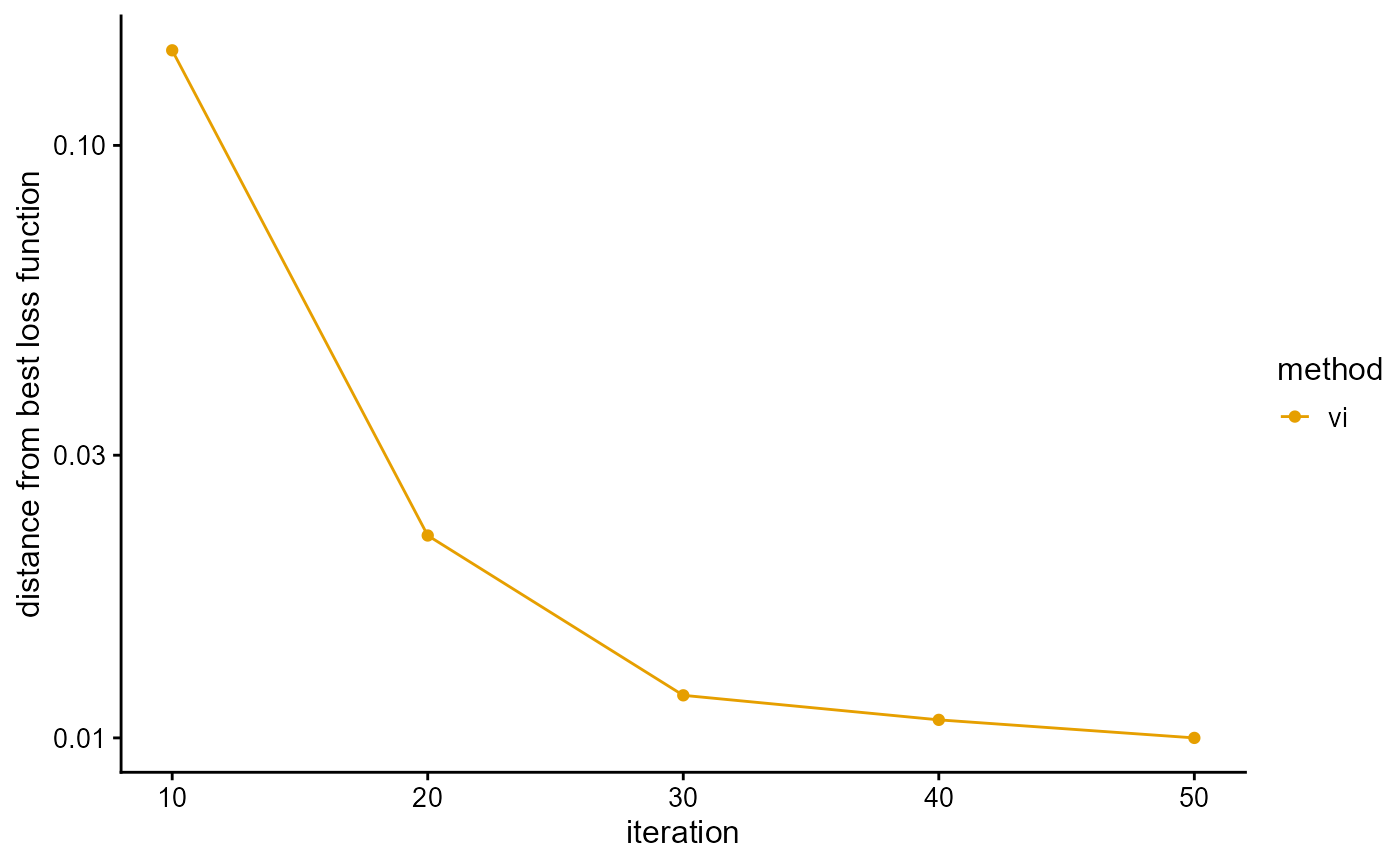

L <- result$Loss
plot_loss(list(L), "vi", 10)

P <- result$P
plot_structure(P)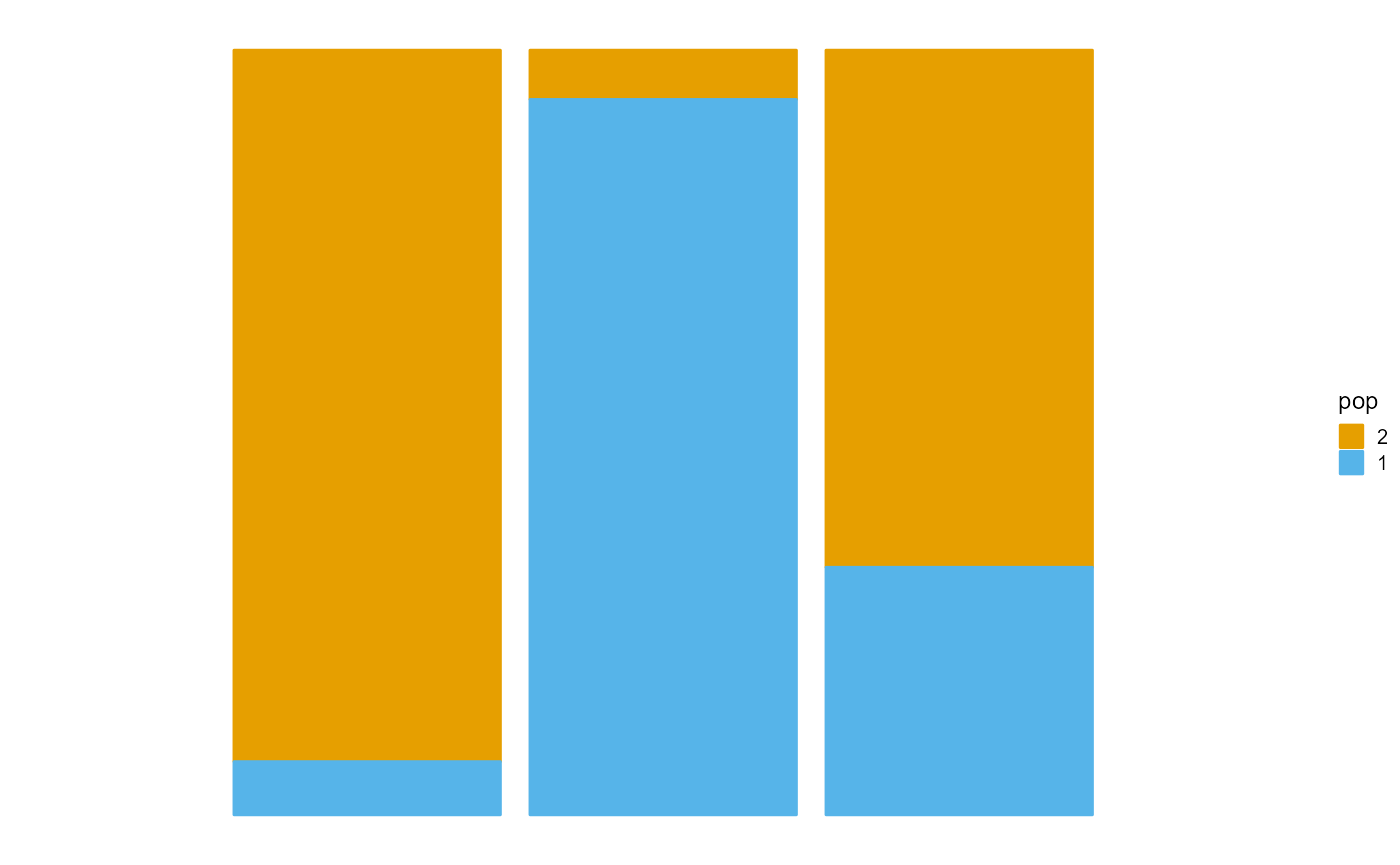

See AwesomePackage for details.

Literature Cited

Blei, David M, Alp Kucukelbir, and Jon D McAuliffe. 2017. “Variational Inference: A Review for Statisticians.” Journal of the American Statistical Association 112 (518): 859–77.

Raj, Anil, Matthew Stephens, and Jonathan K Pritchard. 2014. “fastSTRUCTURE: Variational Inference of Population Structure in Large SNP Data Sets.” Genetics 197 (2): 573–89.

Jonathon Chow

2022-10-04